Data correction

In addition to the raw data importation, which is done similarly to the IDL readomega, OMEGA-Py also includes build-in functions to perform the atmospheric and thermal corrections on a previously loaded OMEGAdata object, using methods described for instance in Jouglet et al. (2007)¹ or Langevin et al. (2005)².

Illustration of the atmospheric and thermal corrections applied to an OMEGA spectrum (figure 1 from Stcherbinine et al., 2021)[^3].

In the following, we assume that we have already loaded an OMEGA observation as follows:

import omegapy.omega_data as od

omega = od.OMEGAdata('0967_3')

Atmospheric correction

The atmospheric correction of a data cube is performed using the volcano-scan technique, by scaling a typical atmospheric spectrum from the 2 μm CO₂ atmospheric band (Langevin et al., 2005)².

Info

Upcoming versions will allow the user to use a custom atmospheric spectrum instead of the one currently provided.

Two methods are available to scale the atmospheric spectrum:

Method 1

The first method (mostly used) adjust the atmospheric scaling to force the values of the reflectance at 1.93 and 2.01 μm to be the same.

omega_corr_atm = od.corr_atm(omega)     # Method 1

Method 2

The second method (less used) adjust the atmospheric scaling to have the "flattest" spectra between 1.93 and 2.00 μm. As it requires a call to a minimization function, the computation time for this method is longer than for the first one.

omega_corr_atm2 = od.corr_atm2(omega)   # Method 2

Thermal correction

If the thermal contribution of the planet in the OMEGA spectra can be neglected for wavelength smaller than ~3 μm, it has to be taken into account when using larger wavelength (i.e., data from the L-channel ; see figure above).

The thermal correction can also be performed using two methods. However, only the first one has been optimized to use multiprocessing for now.

Method 1 (with C-channel)

The reflectance at 5 μm is theoretically estimated from the measured reflectance at 2.4 μm, using typical spectra of the bright and dark regions of Mars from Calvin (1997)⁴. Then the additional black body component is derived and substracted to the entire spectrum (Jouglet et al., 2007)¹.

In addition, to reduce the computation time of the thermal correction, parallel processing has been implemented using the multiprocessing module for this method.

omega_corr_them = od.corr_therm(omega, npool=1)     # Method 1 with 1 single process
# or
omega_corr_them = od.corr_therm(omega, npool=10)    # Method 1 with 10 simultaneous processes

Using multiple processes

npool controls the number of simultaneous processes used to compute the thermal correction of the OMEGA data cube. I.e., it defines the number of multiprocessing.Pool that will be created.

Method 2 (without C-channel)

If the data from the C-channel are not available, the first method is no longer usable, and it is necessary to fit both the surface temperature ad the reflectance at 5 μm, as described in Audouard (2014)⁵.

omega_corr_them2 = od.corr_therm2(omega)            # Method 2

Simultaneous atmospheric & thermal corrections

For the analysis of data from the L-channel, that requires thermal and atmospheric correction of the spectra, one can performs both corrections at the same time with a dedicated function. This is the recommended way if you want to perform both corrections as the atmosphere will be better taken into account while removing the thermal correction.

Method 1 (with C-channel)

For now, only the use of both methods 1 for the atmospheric and thermal corrections has been implemented.

omega_corr_them_atm = od.corr_therm_atm(omega, npool=10)    # Method 1-1

Using multiple processes

npool controls the number of simultaneous processes used to compute the thermal correction of the OMEGA data cube. I.e., it defines the number of multiprocessing.Pool that will be created.

Correcting and saving OMEGA observations in one single command

As the correction of an OMEGA observation can take some time, you may want to save the final cube to avoid reprocessing it every time.

Instead of returning an OMEGAdata object after processing the thermal & atmospheric corrections, it is also possible to save it into a file that can be loaded later using the corr_save_omega2 function (more details here).

Checking applied corrections

The correction status of an OMEGAdata object can be checked via the value of the booleans:

omega.therm_corr    # True if thermal correction applied

omega.atm_corr      # True if atmospheric correction applied

Alternatively, these informations are also displayed in the interactive representation of the object.

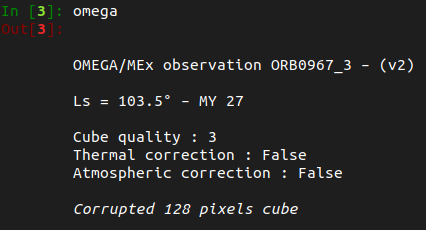
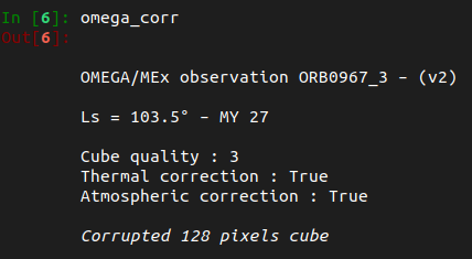
(left) No corrections applied. (right) Both corrections applied.

The informations about the method applied for the corrections can be accessed via:

omega.therm_corr_infos

omega.atm_corr_infos

---

1. D. Jouglet, F. Poulet, R. E. Milliken, et al. (2007). Hydration state of the Martian surface as seen by Mars Express OMEGA : 1. Analysis of the 3 μm hydration feature. Journal of Geophysical Research: Planets, 112, E08S06. doi:10.1029/2006JE002846 ↩↩

2. Y. Langevin, F. Poulet, J.-P. Bibring & B. Gondet (2005). Sulfates in the North Polar Region of Mars Detected by OMEGA/Mars Express. Science, 307, 1584-1586. doi :10.1126/science.1109091 ↩↩

3. A. Stcherbinine, M. Vincendon, F. Montmessin, P. Beck (2021). Identification of a new spectral signature at 3 µm over Martian northern high latitudes: implications for surface composition. Icarus, 369, 114627. doi:10.1016/j.icarus.2021.114627 ↩

4. W. N. Calvin (1997). Variation of the 3-μm absorption feature on Mars : Observations over eastern Valles Marineris by the Mariner 6 infrared spectrometer. Journal of Geophysical Research: Planets, 102, 9097. doi:10.1029/96JE03767 ↩

5. J. Audouard (2014). PhD thesis, Université Paris-Sud XI. ↩